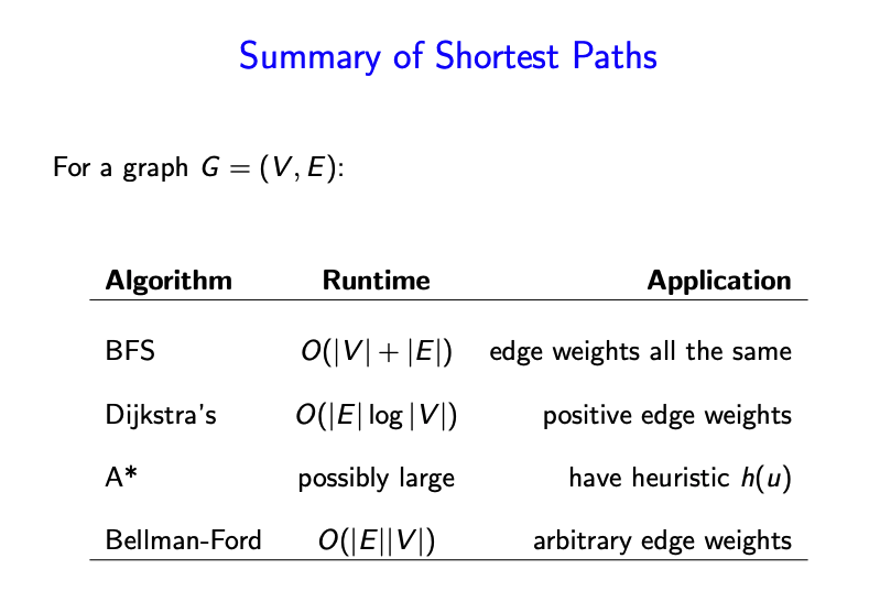
Shortest path problem review

Bellman-ford algorithm

Negative weights

Negative cycles: if some cycle has a negative total cost, we can make the s-t path as low cost as we want

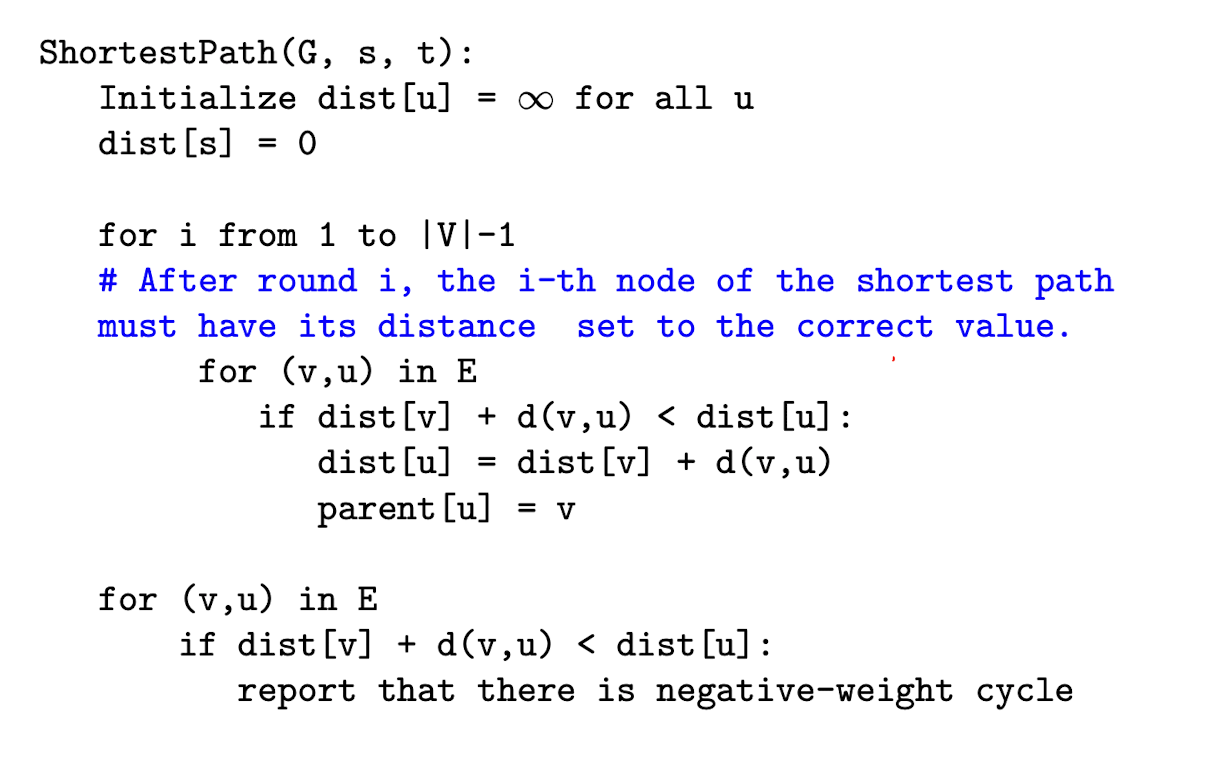
Bellman-ford

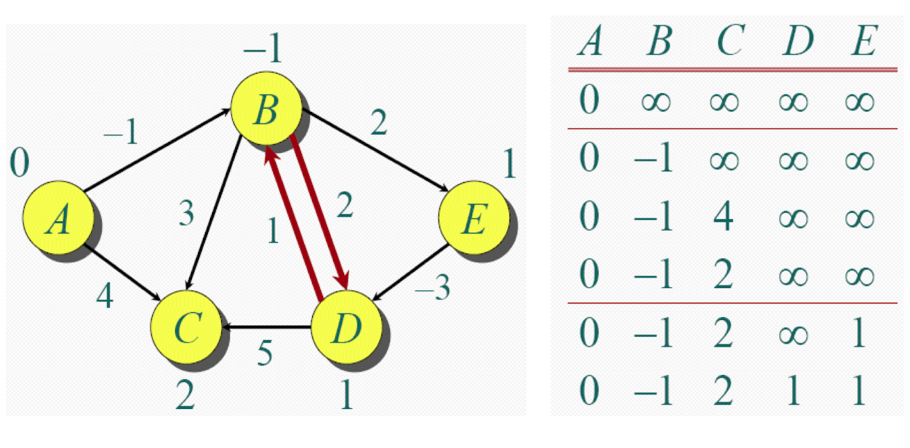
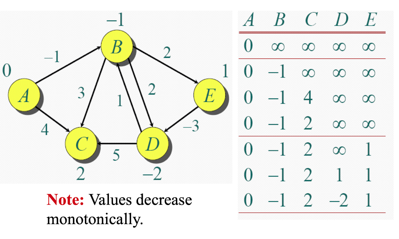
Ford step

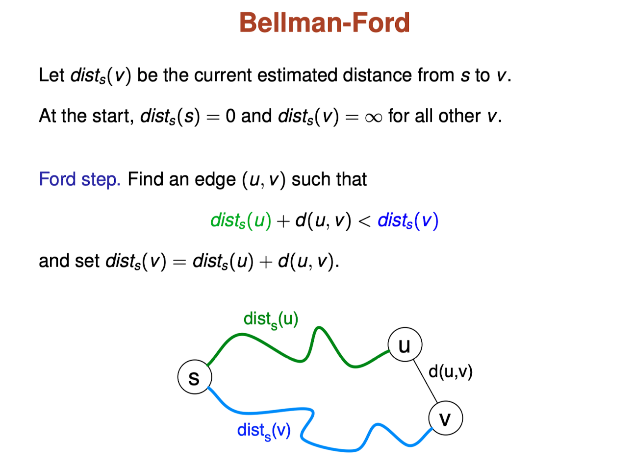
Repeatedly applying Ford Step

Theorem:

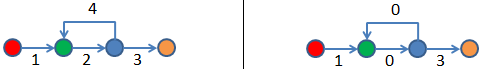
After applying the ford step until for all edges, will equal the shortest-path distance from s to u for all u.

Relaxation procedure

The main operation for all SSSP algorithms discussed in this visualization is the relax(u, v, w(u, v)) operation with the following pseudo-code:

relax(u, v, w_u_v)
  if D[v] > D[u]+w_u_v // if the path can be shortened
    D[v] = D[u]+w_u_v // we 'relax' this edge
    p[v] = u // remember/update the predecessor
    // update some other data structure(s) as necessary

For example, see relax(1,2,4) operation on the figure below: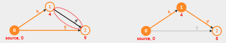 relax operation example

Demo

Report negative cycle

Proof

`Theorem 1`

: If G = (V, E) contains no negative weight cycle, then the shortest path p from source vertex s to a vertex v must be a simple path.

Recall: A simple path is a path p = {v0, v1, v2, …, vk}, (vi, vi+1) ∈ E, ∀ 0 ≤ i ≤ (k-1) and there is no repeated vertex along this path.

Suppose the shortest path p is not a simple path
Then p must contains one (or more) cycle(s) (by definition of non-simple path)
Suppose there is a cycle c in p with positive weight (e.g. green → blue → green on the left image)
If we remove c from p, then we will have a shorter ‘shortest path’ than our shortest path p
A glaring contradiction, so p must be a simple path
Even if c is actually a cycle with zero (0) total weight — it is possible according to our Theorem 1 assumption: no negative weight cycle (see the same green → blue → green but on the right image), we can still remove c from p without increasing the shortest path weight of p
In conclusion, p is a simple path (from point 5) or can always be made into a simple path (from point 6)

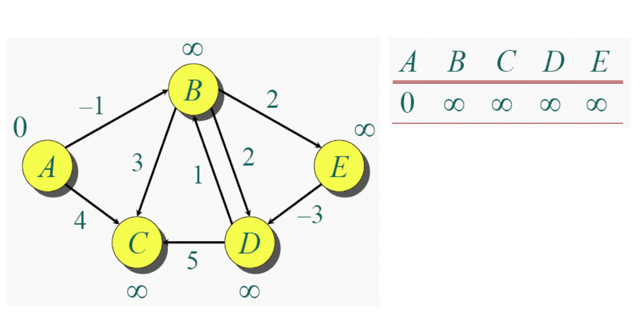
In another word, shortest path p has at most |V|-1 edges from the source vertex s to the ‘furthest possible’ vertex v in G (in terms of number of edges in the shortest path — see the Bellman Ford’s Killer example above).

`Theorem 2:`

If G = (V, E) contains no negative weight cycle, then after Bellman Ford’s algorithm terminates, we will have D[v] = δ(s, u), ∀ u ∈ V.

For this, we will use Proof by Induction and here are the starting points:

Consider the shortest path p from source vertex s to vertex vi where vi is defined as a vertex which the actual shortest path to reach it requires i hops (edges) from source vertex s.

Recall from Theorem 1 that p will be simple path as we have the same assumption of no negative weight cycle.

Initially, D[v0] = δ(s, v0) = 0, as v0 is just the source vertex s
After 1 pass through E, we have D[v1] = δ(s, v1)
After 2 pass through E, we have D[v2] = δ(s, v2)
…
After k pass through E, we have D[vk] = δ(s, vk)
When there is no negative weight cycle, the shortest path p is a simple path (see Theorem 1), thus the last iteration should be iteration |V|-1
After |V|-1 pass through E, we have D[v|V|-1] = δ(s, v|V|-1), regardless the ordering of edges in E — see the Bellman Ford’s Killer example above

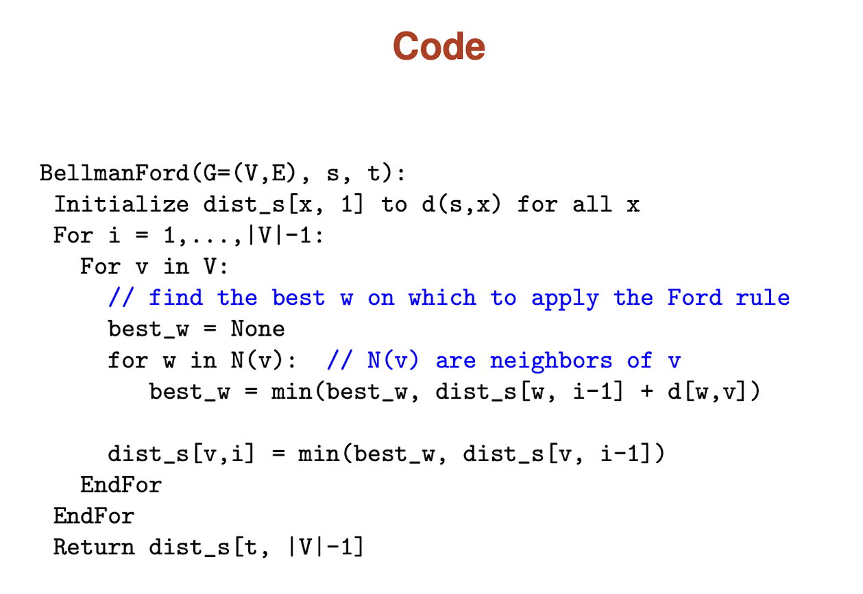
Pseudocode

Queue-based implementation

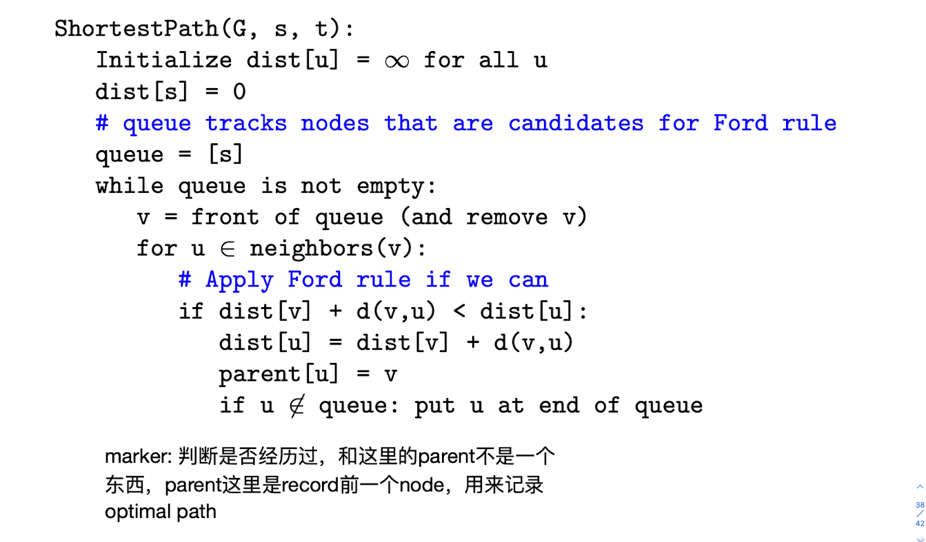
Typical implementation

Dynamic programming

The Bellman-Ford Algorithm is a dynamic programming algorithm for the single-sink (or singlesource) shortest path problem.

It is slower than Dijkstra’s algorithm, but can handle negative weight directed edges, so long as there are no negative-weight cycles.

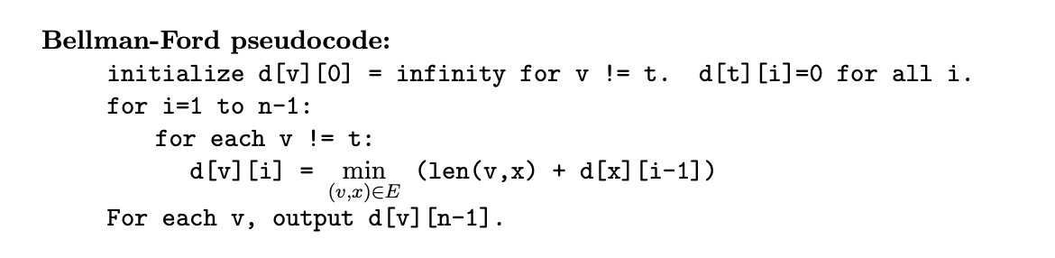
First of all, let’s just compute the lengths of the shortest paths first, and afterwards we can use these lengths to easily reconstruct the paths themselves.

Next, to use Dynamic Programming, we need to define subproblems. The subproblems here will be finding the shortest path from each node v to t that uses i or fewer edges, if such a path exists.

More specifically, the algorithm is as follows:

For each node v, find the length of the shortest path to t that uses at most 1 edge, or write down ∞ if there is no such path.

This is easy: if v = t we get 0; if (v, t) ∈ E then we get len(v, t); else just put down ∞.

Now, suppose for all v we have solved for length of the shortest path to t that uses i − 1 or fewer edges. How can we use this to solve for the shortest path that uses i or fewer edges?

Answer: the shortest path from v to t that uses i or fewer edges will first go to some neighbor x of v, and then take the shortest path from x to t that uses i−1 or fewer edges, which we’ve already solved for! So, we just need to take the min over all neighbors x of v.

How far do we need to go? Answer: at most i = n − 1 edges. Why? Because more than that will create a cycle, and we can then just cut out the cycle to get a shorter path (remember there are no negative-weight cycles).

Specifically, here is pseudocode for the algorithm. We will use d[v][i] to denote the length of the shortest path from v to t that uses i or fewer edges (if it exists) and infinity otherwise (“d” for “distance”). Also, for convenience we will use a base case of i = 0 rather than i = 1

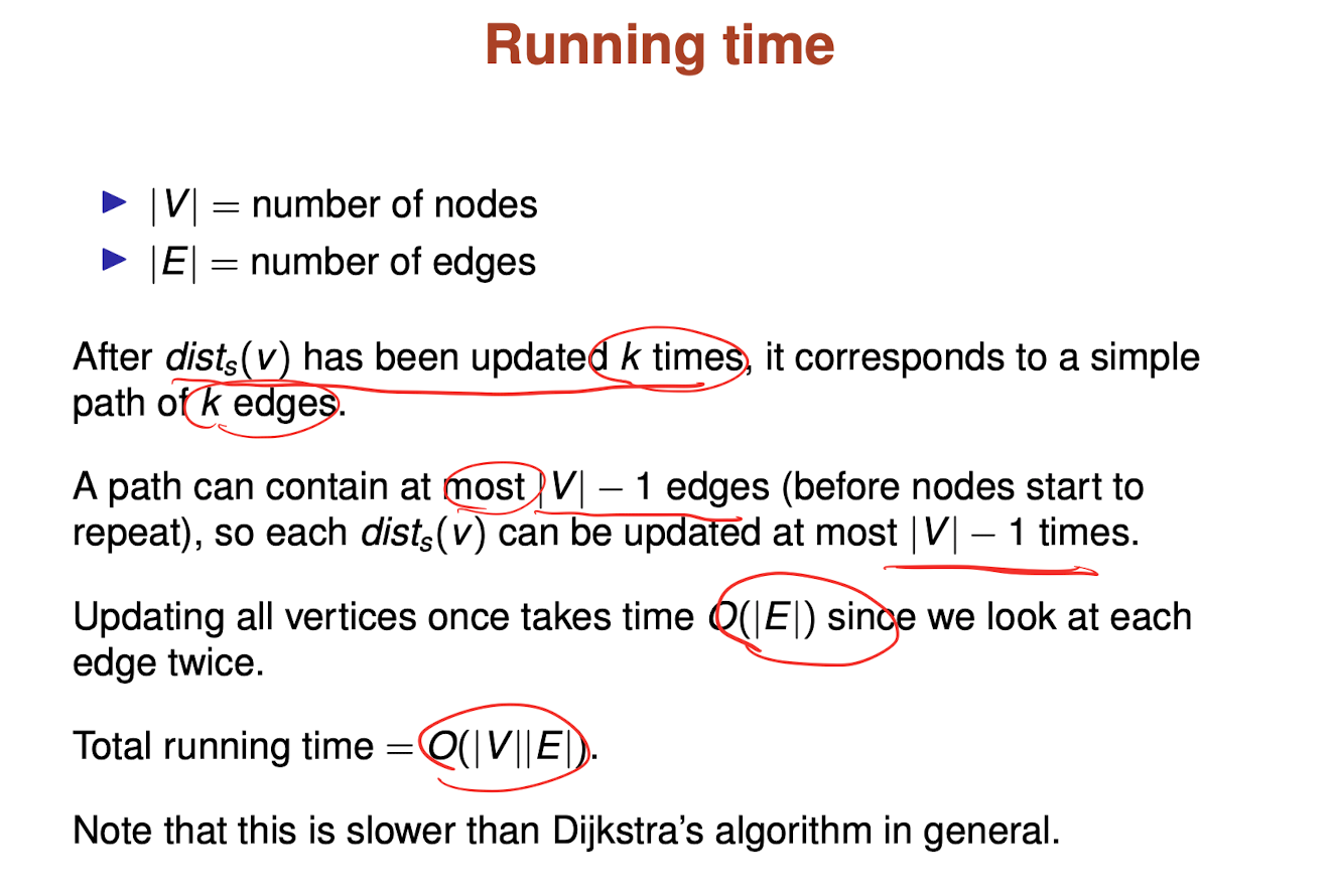
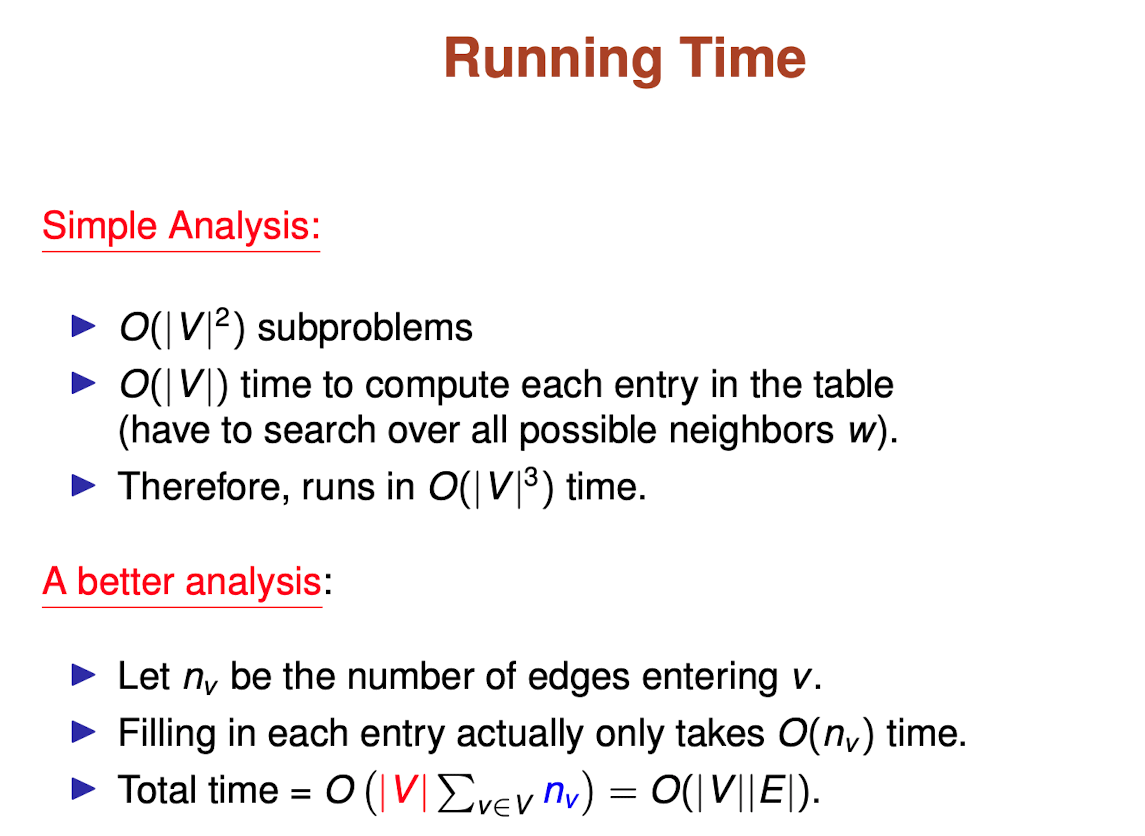
Run time analysis

Bellman Ford’s &Dijkstra’s

Bellman Ford’s algorithm

Like other Dynamic Programming Problems, the algorithm calculates shortest paths in a bottom-up manner.

It first calculates the shortest distances which have at-most one edge in the path.
Then, it calculates the shortest paths with at-most 2 edges, and so on.
After the i-th iteration of outer loop, the shortest paths with at most i edges are calculated.

There can be maximum |V| – 1 edge in any simple path, that is why the outer loop runs |v| – 1 time.

The idea is, assuming that there is no negative weight cycle if we have calculated shortest paths with at most i edges, then an iteration over all edges guarantees to give the shortest path with at-most (i+1) edges

Dijkstra’s algorithm

Dijkstra’s algorithm is very similar to Prim’s algorithm for minimum spanning tree. Like Prim’s MST, we generate an SPT (shortest path tree) with a given source as root.

We maintain two sets, one set contains vertices included in the shortest-path tree, other set includes vertices not yet included in the shortest-path tree. At every step of the algorithm, we find a vertex which is in the other set (set of not yet included) and has a minimum distance from the source.

Bellman Ford’s Algorithm	Dijkstra’s Algorithm
Bellman Ford’s Algorithm works when there is negative weight edge, it also detects the negative weight cycle.	Dijkstra’s Algorithm doesn’t work when there is negative weight edge.
The result contains the vertices which contains the information about the other vertices they are connected to.	The result contains the vertices containing whole information about the network, not only the vertices they are connected to.
It can easily be implemented in a distributed way.	It can not be implemented easily in a distributed way.
It is more time consuming than Dijkstra’s algorithm. Its time complexity is O(VE).	It is less time consuming. The time complexity is O(E logV).
Dynamic Programming approach is taken to implement the algorithm.	Greedy approach is taken to implement the algorithm.