Key notes for Deep learning in new computational modeling techniques for genomics

Cross-linking immunoprecipitation (CLIP) is a method used in molecular biology that combines UV cross-linking with immunoprecipitation in order to analyze protein interactions with RNA or to precisely locate RNA modifications (e.g. m6A). CLIP-based techniques can be used to map RNA binding protein binding sites or RNA modification sites of interest on a genome-wide scale, thereby increasing the understanding of post-transcriptional regulatory networks.

Feature

An individual, measurable property or characteristic of a phenomenon being observed.

Handcrafted features

Features derived from raw data (or other features) using manually specified rules. Unlike learned features, they are specified upfront and do not change during model training. For example, the GC content is a handcrafted feature of a DNA sequence.

End-to-end models

Machine learning models that embed the entire data-processing pipeline to transform raw input data into predictions without requiring a preprocessing step.

Deep neural networks

A wide class of machine learning models with a design that is loosely based on biological neural networks.

Fully connected

Referring to a layer that performs an affine transformation of a vector followed by application of an activation function to each value.

Convolutional

Referring to a neural network layer that processes data stored in n-dimensional arrays, such as images. The same fully connected layer is applied to multiple local patches of the input array. When applied to DNA sequences, a convolutional layer can be interpreted as a set of position weight matrices scanned across the sequence.

Recurrent

Referring to a neural network layer that processes sequential data. The same neural network is applied at each step of the sequence and updates a memory variable that is provided for the next step.

Graph convolutional

Referring to neural networks that process graph-structured data; they generalize convolution beyond regular structures, such as DNA sequences and images, to graphs with arbitrary structures. The same neural network is applied to each node and edge in the graph.

Autoencoders

Unsupervised neural networks trained to reconstruct the input. One or more bottleneck layers have lower dimensionality than the input, which leads to compression of data and forces the autoencoder to extract useful features and omit unimportant features in the reconstruction.

Generative adversarial networks

(GANs). Unsupervised learning models that aim to generate data points that are indistinguishable from the observed ones.

Target

The desired output used to train a supervised model.

Loss function

A function that is optimized during training to fit machine learning model parameters. In the simplest case, it measures the discrepancy between predictions and observations. In the case of quantitative predictions such as regression, mean-squared error loss is frequently used, and for binary classification, the binary cross-entropy, also called logistic loss, is typically used.

k\-mer

Character sequence of a certain length. For instance, a dinucleotide is a k-mer for which k = 2.

Logistic regression

A supervised learning algorithm that predicts the log-odds of a binary output to be of the positive class as a weighted sum of the input features. Transformation of the log-odds with the sigmoid activation function leads to predicted probabilities.

Sigmoid function

A function that maps real numbers to [0,1], defined as 1/(1 + e −x).

Activation function

A function applied to an intermediate value x within a neural network. Activation functions are usually nonlinear yet very simple, such as the rectified-linear unit or the sigmoid function.

Regularization

A strategy to prevent overfitting that is typically achieved by constraining the model parameters during training by modifying the loss function or the parameter optimization procedure. For example, the so-called L2 regularization adds the sum of the squares of the model parameters to the loss function to penalize large model parameters.

Hidden layers

Layers are a list of artificial neurons that collectively represents a function that take as input an array of real numbers and returns an array of real numbers corresponding to neuron activations. Hidden layers are between the input and output layers.

Rectified-linear unit

(ReLU). Widely used activation function defined as max(0, x).

Neuron

The elementary unit of a neural network. An artificial neuron aggregates the inputs from other neurons and emits an output called activation. Inputs and activations of artificial neurons are real numbers. The activation of an artificial neuron is computed by applying a nonlinear activation function to a weighted sum of its inputs.

Linear regression

A supervised learning algorithm that predicts the output as a weighted sum of the input features.

Decision trees

Supervised learning algorithms in which the prediction is made by making a series of decisions of type ‘is feature i larger than x’ (internal nodes of the tree) and then predicting a constant value for all points satisfying the same decisions series (leaf nodes).

Random forests

Supervised learning algorithms that train and average the predictions of many decision trees.

Gradient-boosted decision trees

Supervised learning algorithms that train multiple decision trees in a sequential manner; at each time step, a new decision tree is trained on the residual or pseudo-residual of the previous decision tree.

Position weight matrix

(PWM). A commonly used representation of sequence motifs in biological sequences. It is based on nucleotide frequencies of aligned sequences at each position and can be used for identifying transcription factor binding sites from DNA sequence.

Overfitting

The scenario in which the model fits the training set very well but does not generalize well to unseen data. Very flexible models with many free parameters are prone to overfitting, whereas models with many fewer parameters than the training data do not overfit.

Filters = kernel

Parameters of a convolutional layer. In the first layer of a sequence-based convolutional network, they can be interpreted as position weight matrices.

Pooling operation

A function that replaces the output at a certain location with a summary statistic of the nearby outputs. For example, the max pooling operation reports the maximum output within a rectangular neighbourhood.

Channel

An axis other than one of the positional axes. For images, the channel axis encodes different colours (such as red, green and blue), for one-hot-encoded sequences (A: [1, 0, 0, 0], C: [0, 1, 0, 0] and so on), it denotes the bases (A, C, G and T), and for the output of the convolutions, it corresponds to the outputs of different filters.

Dilated convolutions

Filters that skip some values in the input layers. Typically, each subsequent convolutional layer increases the dilation by a factor of two, thus achieving an exponentially increasing receptive field with each additional layer.

Receptive field

The region of the input that affects the output of a convolutional neuron.

Memory

An array that stores the information of the patterns observed in the sequence elements previously processed by a recurrent neural network.

Feature importance scores

The quantification values of the contributions of features to a current model prediction. The simplest way to obtain this score is to perturb the feature value and measure the change in the model prediction: the larger the change found, the more important the feature is.

Backpropagation

An algorithm for computing gradients of neural networks. Gradients with respect to the loss function are used to update the neural network parameters during training.

Saliency maps

Feature importance scores defined as the gradient absolute values of the model output with respect to the model input.

Input-masked gradients

Feature importance scores defined as the gradient of the model output with respect to the model input multiplied by the input values.

Automatic differentiation

A set of techniques, which consist of a sequence of elementary arithmetic operations, used to automatically differentiate a computer program.

Model architecture

The structure of a neural network independent of its parameter values. Important aspects of model architecture are the types of layers, their dimensions and how they are connected to each other.

k\-means

An unsupervised method for partitioning the observations into clusters by alternating between refining cluster centroids and updating cluster assignments of observations.

Principal component analysis

An unsupervised learning algorithm that linearly projects data from a high-dimensional space to a lower-dimensional space while retaining as much variance as possible.

t-Distributed stochastic neighbour embedding

(t-SNE). An unsupervised learning algorithm that projects data from a high-dimensional space to a lower-dimensional space (typically 2D or 3D) in a nonlinear fashion while trying to preserve the distances between points.

Latent variable models

Unsupervised models describing the observed distribution by imposing latent (unobserved) variables for each data point. The simplest example is the mixture of Gaussian values.

Bottleneck layer

A neural network layer that contains fewer neurons than previous and subsequent layers.

Generative models

Models able to generate points from the desired distribution. Deep generative models are often implemented by a neural network that transforms samples from a standard distribution (normal and uniform) into samples from a complex distribution (gene expression levels or sequences that encode a splice site).

Hyperparameters

Parameters specifying the model or the training procedure that are not optimized by the learning algorithm (for example, by the stochastic gradient descent algorithm). Examples of hyperparameters are the number of layers, regularization strength, batch size and the optimization step size.

one epoch = one forward pass and one backward pass of all the training examples

batch size = the number of training examples in one forward/backward pass. The higher the batch size, the more memory space you’ll need.

number of iterations = number of passes, each pass using [batch size] number of examples. To be clear, one pass = one forward pass + one backward pass (we do not count the forward pass and backward pass as two different passes).

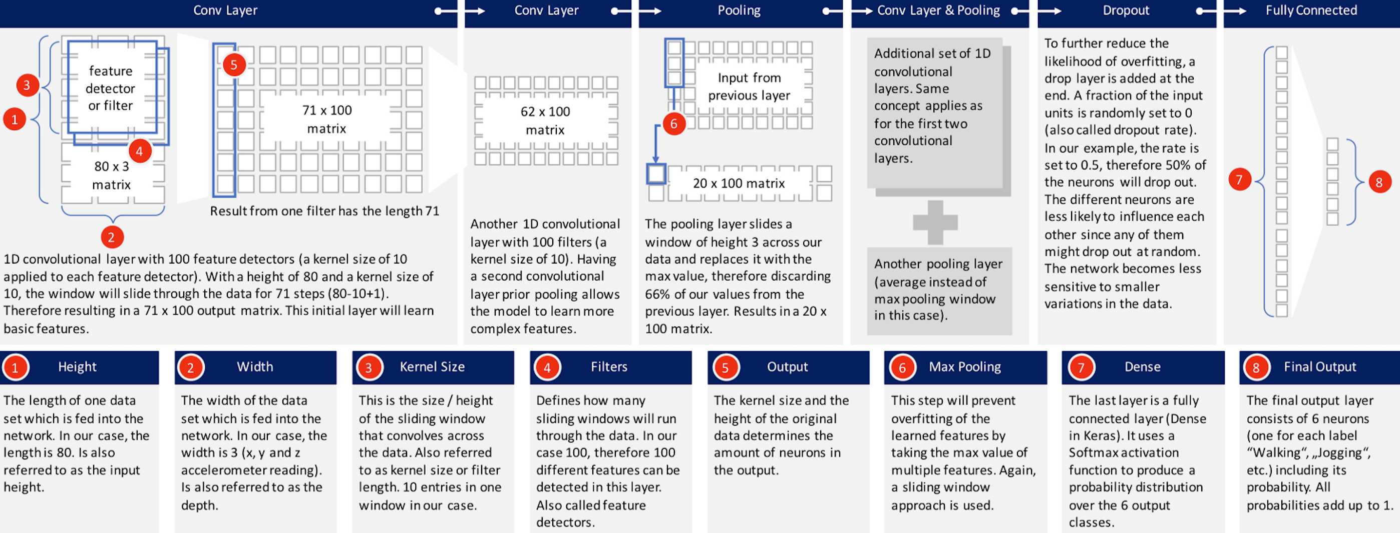
dropout: to further reduce the likelihood of overfitting, a drop layer is added to the end. A fraction of the input units is randomly set to 0 (also called dropout rate). e.g the rate = 0.5, which means 50% of the neurons are less likely to influence each other since any of them might drop out at random. The network becomes less sensitive to smaller variations in the data

dense: The last layer is a fully connected layer (Dense in keras). It uses a Softmax activation function to produce a probability distribution over the n output classes