Cardiovascular diseases (CVDs) are the number 1 cause of death globally, taking an estimated 17.9 million lives each year, which accounts for 31% of all deaths worlwide.
Heart failure is a common event caused by CVDs.
Most cardiovascular diseases can be prevented by addressing behavioural risk factors such as tobacco use, unhealthy diet and obesity, physical inactivity and harmful use of alcohol using population-wide strategies.
People with cardiovascular disease or who are at high cardiovascular risk (due to the presence of one or more risk factors such as hypertension, diabetes, hyperlipidaemia or already established disease) need early detection and management wherein a machine learning model can be of great help.
Project description (overview)
The input to our predictor is is a medical dataset which contains 12 features that can be used to predict mortality by heart failure.
- Data exploration
- Principle Components Analysis (PCA) to reduce the dimension of features to have a view of the input data distribution
- Build a preliminary linear SVM model to incorporate all the features to see the model performance.
- Feature selection part.
- Chi-square test to check the correlation between each categorical feature and the target death event.
- Heat map to return the features with high correlation coefficient with death events.
- Visualized the each feature’s contribution significance in the SVM model
- Compared the returned features and determined the final selected features
- Model comparison and hyperparameter tuning
- compare the performance in difference preprocessing methods MinMaxScalar, StandardScalar, RobustScalar
- compare the performance in k-fold cross validation and leave-one-out methods
- compare the kernel selected in Support Vector Machine (linear or rbf)
- grid search to find the best performance model
- Selected model performance
- calculated the precision, recall, accuracy and f1-score
- plot the ROC and PR-curve
- plot the learning curve
Related work
Explorative data analysis (EDA) approach
Strength: Detailed explorative and associative data analysis with great data visualization: each factor is visualized by different types of figures
Weakness: Prediction model are quite rudimentary, the author did not select the features and tune the models’ hyperparameters.
Similarity: I learned and applied the plotly.express API to create fancy and concise figures for easy comparison; I furthered his rudimentary model by optimization
Predictive data analysis (PDA) approach
Strength: The author compares six prediction models with feature selection. The Extra Gradient Booster Classifier could achieve the accuracy up to 95.0%
Weakness: The author consider the “time” column as the useful features.
Similarity: I don’t think “time” colume should be included since “time” column stands for Follow-up period (days), which means itself could not contribute the diseases itself. Therefore, I consider this feature as uselessness in our prediction model
Strength: The author uses a new method: Chi-square test to find the correlation between single categorical feature with target death_event
Weakness: The visualization part does not as fancy as previous work
Similarity: I learned and used the Chi-square test to conduct the correlation test between single categorical data with the categorical death_event; but i didn’t agree the author’s method in using box plot comparison between numerical data with categorical data, I used heat map instead.
Data download
You could simply download the data from my own Github repository: https://media.githubusercontent.com/media/yuxuanwu17/kaggle/main/heart_failure_clinical_records_dataset.csv
You could also download the data from kaggle:
https://www.kaggle.com/andrewmvd/heart-failure-clinical-data
Libraries used in this project
1 | %matplotlib inline |
Problem formulation
Return the head of dataset (a overview of inside components)
1 | # df = pd.read_csv("/home/yuxuan/kaggle/heart_failure_clinical_records_dataset.csv") |
| age | anaemia | creatinine_phosphokinase | diabetes | ejection_fraction | high_blood_pressure | platelets | serum_creatinine | serum_sodium | sex | smoking | time | DEATH_EVENT | |
|---|---|---|---|---|---|---|---|---|---|---|---|---|---|
| 0 | 75.0 | 0 | 582 | 0 | 20 | 1 | 265000.00 | 1.9 | 130 | 1 | 0 | 4 | 1 |
| 1 | 55.0 | 0 | 7861 | 0 | 38 | 0 | 263358.03 | 1.1 | 136 | 1 | 0 | 6 | 1 |
| 2 | 65.0 | 0 | 146 | 0 | 20 | 0 | 162000.00 | 1.3 | 129 | 1 | 1 | 7 | 1 |
| 3 | 50.0 | 1 | 111 | 0 | 20 | 0 | 210000.00 | 1.9 | 137 | 1 | 0 | 7 | 1 |
| 4 | 65.0 | 1 | 160 | 1 | 20 | 0 | 327000.00 | 2.7 | 116 | 0 | 0 | 8 | 1 |
Print the size of the dataset
1 | print(heart_data.shape) |
(299, 13)Check the ratio of the NaNs for each column
1 | for col in heart_data.columns: |
age 0.0%
anaemia 0.0%
creatinine_phosphokinase 0.0%
diabetes 0.0%
ejection_fraction 0.0%
high_blood_pressure 0.0%
platelets 0.0%
serum_creatinine 0.0%
serum_sodium 0.0%
sex 0.0%
smoking 0.0%
time 0.0%
DEATH_EVENT 0.0%
Dataset description
There are 13 dimensions and 299 samples. All the columns are devoid of NaNs. We need make some rules before the data processing。
Target features (binary classification): DEATH_EVENT
Categorical data
- Sex - Gender of patient Male = 1, Female =0
- Diabetes - 0 = No, 1 = Yes
- Anaemia - 0 = No, 1 = Yes
- High_blood_pressure - 0 = No, 1 = Yes
- Smoking - 0 = No, 1 = Yes
- DEATH_EVENT - 0 = No, 1 = Yes
Numerical data
- Age - Age of patient
- creatinine_phosphokinase - Level of the CPK enzyme in the blood (mcg/L)
- ejection_fraction - Percentage of blood leaving the heart at each contraction (percentage)
- platelets - Platelets in the blood (kiloplatelets/mL)
- serum_creatinine - Level of serum creatinine in the blood (mg/dL)
- serum_sodium - Level of serum sodium in the blood (mEq/L)
- time - Follow-up period (days)
Citation or Reference
Dataset from Davide Chicco, Giuseppe Jurman: Machine learning can predict survival of patients with heart failure from serum creatinine and ejection fraction alone. BMC Medical Informatics and Decision Making 20, 16 (2020)
The dataset downloaded from Kaggle https://www.kaggle.com/andrewmvd/heart-failure-clinical-data
Principle components analysis
Reduce the dimensions and return the sample distribution
1 | %matplotlib inline |
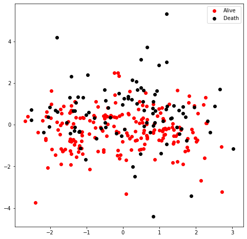
I would like to have a view of the sample distribution in the dataset. Therefore, I used the principle component analysis (PCA) to reduce the dimension of features into 2D for visualization. The figure suggested that the data are densed and not easy to seperate (either linear or non-linear model), indicating the existence of insignificant feature which could negatively influence the future prediction accuracy.
Correlation analysis
I would like to find the correlation between each feature, especially with the target variable: DEATH_EVENT.
In this case, I excluded the column “time” since the time tracked could not contribute to the heart failure itself.
1 | import seaborn as sn |

Data partition
- As I mentioned before, I will not take the feature “time” into consideration. Therefore, 11 features are included in the final model prediction.
- I split the dataset into two categories. 80% for raining data and 20% for testing data.
- I used the StandardScalar normalization method to preprocess the data
1 | from sklearn.preprocessing import StandardScaler |
The number of training sample is 239
The number of testing sample is 60
Feature selection (feature engineering)
Method 1: Chi-square test
- Based on previous research, I could conclude that DEATH_EVENT is our target. Since I have six categorical data I would like to figure out whether these single categorical valuable has significant correlation with the DEATH_EVENT.
- Crosstables/contingency tables are one of the best ways to see how categorical variables are distributed among each other.
- The following test suggests that we failed to reject the $H_0$ problem, indicating that there is no direct relationship between the DEATH_EVENT
1 | import pandas as pd |
————————————–
CROSSTAB BETWEEN ANAEMIA & DEATH_EVENT
————————————–
anaemia 0 1
DEATH_EVENT
0 120 83
1 50 46
H0: THERE IS NO RELATIONSHIP BETWEEN DEATH_EVENT & ANAEMIA
H1: THERE IS RELATIONSHIP BETWEEN DEATH_EVENT & ANAEMIA
P-VALUE: 0.31
FAILED TO REJECT H0
—————————————
CROSSTAB BETWEEN DIABETES & DEATH_EVENT
—————————————
diabetes 0 1
DEATH_EVENT
0 118 85
1 56 40
H0: THERE IS NO RELATIONSHIP BETWEEN DEATH_EVENT & DIABETES
H1: THERE IS RELATIONSHIP BETWEEN DEATH_EVENT & DIABETES
P-VALUE: 0.93
FAILED TO REJECT H0
————————————————–
CROSSTAB BETWEEN HIGH_BLOOD_PRESSURE & DEATH_EVENT
————————————————–
high_blood_pressure 0 1
DEATH_EVENT
0 137 66
1 57 39
H0: THERE IS NO RELATIONSHIP BETWEEN DEATH_EVENT & HIGH_BLOOD_PRESSURE
H1: THERE IS RELATIONSHIP BETWEEN DEATH_EVENT & HIGH_BLOOD_PRESSURE
P-VALUE: 0.21
FAILED TO REJECT H0
———————————-
CROSSTAB BETWEEN SEX & DEATH_EVENT
———————————-
sex 0 1
DEATH_EVENT
0 71 132
1 34 62
H0: THERE IS NO RELATIONSHIP BETWEEN DEATH_EVENT & SEX
H1: THERE IS RELATIONSHIP BETWEEN DEATH_EVENT & SEX
P-VALUE: 0.96
FAILED TO REJECT H0
————————————–
CROSSTAB BETWEEN SMOKING & DEATH_EVENT
————————————–
smoking 0 1
DEATH_EVENT
0 137 66
1 66 30
H0: THERE IS NO RELATIONSHIP BETWEEN DEATH_EVENT & SMOKING
H1: THERE IS RELATIONSHIP BETWEEN DEATH_EVENT & SMOKING
P-VALUE: 0.93
FAILED TO REJECT H0
——————————————
CROSSTAB BETWEEN DEATH_EVENT & DEATH_EVENT
——————————————
DEATH_EVENT 0 1
DEATH_EVENT
0 203 0
1 0 96
H0: THERE IS NO RELATIONSHIP BETWEEN DEATH_EVENT & DEATH_EVENT
H1: THERE IS RELATIONSHIP BETWEEN DEATH_EVENT & DEATH_EVENT
P-VALUE: 0.0
REJECT H0
Method 2: correlation analysis
- Use correlation coefficient > 0.1 with death event
- This method is applicable for both categorical data and numerical data
1 | feature_corr = heart_data.corr() |
age                  0.253729
ejection_fraction   -0.268603
serum_creatinine     0.294278
serum_sodium        -0.195204
time                -0.526964
DEATH_EVENT          1.000000
Name: DEATH_EVENT, dtype: float64
Method 3: Visualized plots of feature importance in linear SVM
1 | import numpy as np |
1 | from sklearn.svm import LinearSVC |
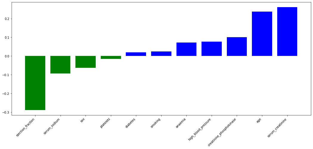
- The ahead plot illustrates the importance of feature in SVM model. y axis could be considered as weights and the absolute value of weights could suggest the contribution to the final results.
- The correlation analysis between factors and death event returned the coefficient > 0.1 features
- Both analysis returned three same features: serum_creatinine, age, ejection_fraction
- we need to evaluate and compare the performance in serum_sodium and creatinine_phosphokinase
1 | from sklearn.svm import SVC |
Accuracy of linear SVM model with feature serum_sodium is : 81.67%
Accuracy of linear SVM model with feature creatinine_phosphokinase is : 83.33%
Therefore, four features including serum_creatinine, age, ejection_fraction, creatinine_phosphokinase
Visualized the learning curve after feature selection
1 | from sklearn.model_selection import learning_curve |
1 | fig, axes = plt.subplots(3, 2, figsize=(10, 15)) |
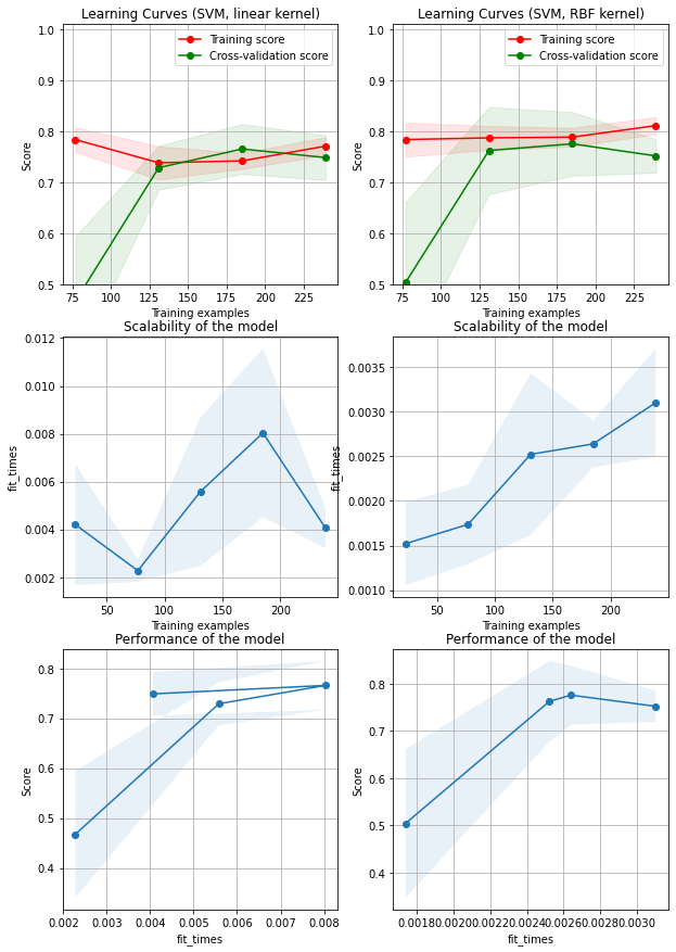
First column is the combination of learning curves, model scability, model performance in a SVM model with linear kernel. First row is the learning curve of linear SVM model: the training score is very high at the beginning and decreases and the cross-validation score is very low at the beginning and increases. The training score and the cross-validation score intertwines at about 220 training samples, and their difference after that are not significant
Second column is the combination of learning curves, model scability, model performance in a SVM model with linear kernel. The learning curve plots indicate that accuracy for both training score and cross validation score tend to be stable after 130 samples, which is similar in linear SVM model. The fit time for RBF kernel SVM is higher than linear kernel because of the complexity in calculation
RBF kernel has a relative higher performance, but the difference is not significant
The figure above doesn’t indicate either overfitting or underfitting problems
Explorative data analysis of the four selected features:
- ‘serum_creatinine’
- ‘age’
- ‘ejection_fraction’
- ‘creatinine_phosphokinase’
Specify the figure size
1 | HEIGHT = 500 |
1 | ## Define the histogram |
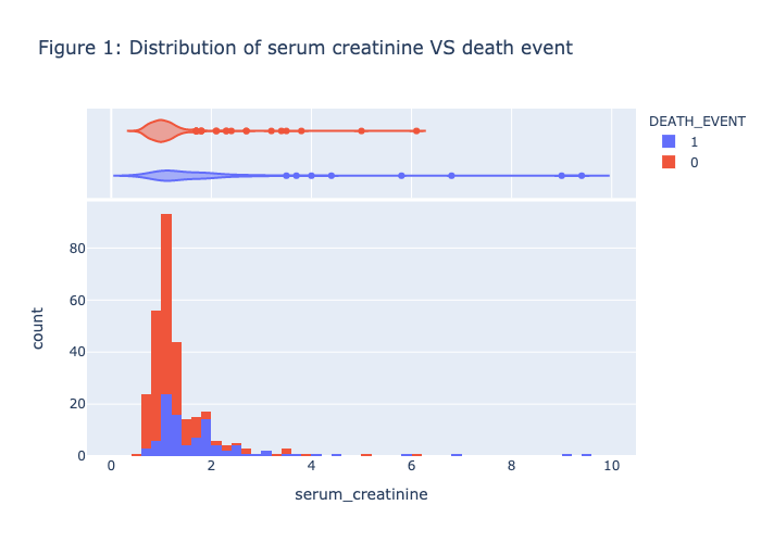
1 | plot_histogram(heart_data, 'serum_creatinine', 'DEATH_EVENT', NBINS, "violin",'Figure 1: Distribution of serum creatinine VS death event') |
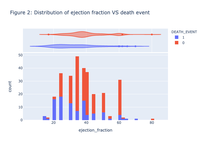
1 | plot_histogram(heart_data, 'ejection_fraction', 'DEATH_EVENT', NBINS, "violin",'Figure 2: Distribution of ejection fraction VS death event') |
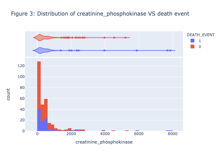
1 | plot_histogram(heart_data, 'creatinine_phosphokinase', 'DEATH_EVENT', NBINS, "violin",'Figure 3: Distribution of creatinine_phosphokinase VS death event') |
1 | import plotly.graph_objs as go |
1 | ## Define the violin plot function method |
1 | violin_boxplot(heart_data,x = "sex",y="age",color="DEATH_EVENT",points="all",box=True,hover_data=heart_data.columns) |
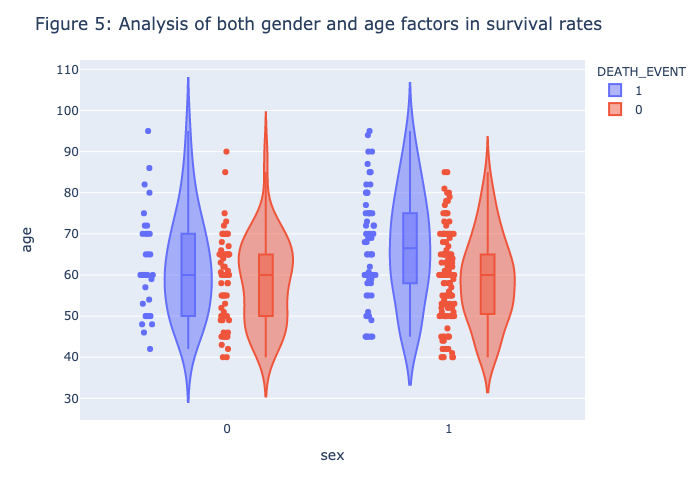
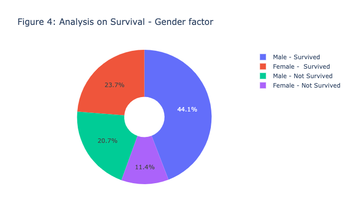
Figure 1 - Figure 5 is the visualization of each feature, there is no clear patterns or strong association between the death_event. Therefore, we need to further our research by conducting the model prediction process.
Methods
Python library
Description: how you learned the predictor
1 | from sklearn.decomposition import PCA |
PCA to visualize the sample distribution
1 | pca = PCA(n_components=2) |
<matplotlib.legend.Legend at 0x7fdff0ee0d90>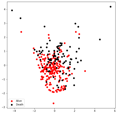
In this case, the data distribution after feature selection are scattered, which could be beneficial for separation. Still, we could not determine whether linear kernel or RBF kernel is suitable for classification. I then would compare the performance between these two methods.
Machine learning algorithms with description
SVM with linear kernel
$$ K(x,y) = X^Ty=x\cdot y$$
Loss function: hinge loss / squared hinge loss
$$ Agreement: z = y_i(w \cdot x_i + \alpha) $$
Hinge loss
$$
L_h(z)= \begin{cases}
0 & \text{if z$\geq$1}\
1-z & \text{z<1}
\end{cases}
$$
Squared hinge loss
$$
L_{hsqr}(z)= \begin{cases}
0 & \text{if z$\geq$1}\
(1-z)^2 & \text{z<1}
\end{cases}
$$
Optimization objective formula for hinge loss:
$$
J(w,\alpha) = \frac{1}{n}\sum_{i=1}^nL_h(y_i(w\cdot x_i + \alpha))+\frac{\lambda}{2}(||w||)^2
$$
Description:
- Linear Kernel is used when the data is linearly separable dataset.
- One of the goal is to minimize the previous objective formula for the hinge loss. $\lambda$ in this case stands for the regularization hyperparameter.
- The strength of the regularization is inversely proportional to $\lambda$, it has to be strictly positive. The smaller regularization parameter means less tolerant to misclassification.
- Require grid serach to return the suitable hyperparameter
SVM with RBF kernel
$$ K(x,y) = e^{-\gamma||x-y||^2}, \gamma >0 $$
Loss function: hinge loss / squared hinge loss
$$ Agreement: z = y_i(w \cdot \phi(x_i) + \alpha) $$
Hinge loss
$$
L_h(z)= \begin{cases}
0 & \text{if z$\geq$1}\
1-z & \text{z<1}
\end{cases}
$$
Squared hinge loss
$$
L_{hsqr}(z)= \begin{cases}
0 & \text{if z$\geq$1}\
(1-z)^2 & \text{z<1}
\end{cases}
$$
Optimization objective formula for hinge loss:
$$
J(w,\alpha) = \frac{1}{n}\sum_{i=1}^nL_h(y_i(w\cdot \phi(x_i) + \alpha))+\frac{\lambda}{2}(||w||)^2
$$
Description:
- SVM with RBF kernel was utilized to solve the linearly inseparable probelms
- kernel trick was used in RBF kernel SVM to increase the computational efficiency
- $\gamma$ parameter how far the influence of a single training example reaches
- C parameter trades off correct classification of training examples against maximization of the decision function’s margin
Evaluation method
Mean squared error (MSE)
$$
MSE = \frac{1}{n}\sum_{i=1}^n(Y_i- \hat{Y_i})^2
$$
where $Y_i$ is the label and $\hat{Y_i}$ is the predicted label by model
1 | heart_data = df.copy() |
Accuracy of linear SVM model is : 83.33%
Mean squared error of linear SVM model is : 0.17
Accuracy of RBF SVM model is : 86.67%
Mean squared error of linear SVM model is : 0.13
Experiments and results
Compare the efficacy of different preprocessing methods
- MinMaxScalar
- StandardScalar
- RobustScalar
1 | from sklearn.pipeline import Pipeline |
Test score for MinMaxScalar RBF kernel: 0.850
Test score for MinMaxScalar linear kernel: 0.767

Test score for StandardScalar in RBF kernel: 0.850
Test score for StandardScalar in linear kernel: 0.833

Test score for RobustScalar in RBF kernel: 0.800
Test score for RobustScalar in linear kernel: 0.817- There is no significant difference between different preprocessing method in RBF kernels, especially in MinMaxScalar and StandardScalar.
- Overall RBF kernel outperforms than linear kernel.
- In this case, I would insist on using StandardScalar in following procedure.
Compare the model performance by ten-fold cross validation and leave-one-out method in model evaluation
Owing to the fact that the dataset I used is a small one, only containing 299 samples in total. In order to minimize the bias or error leading by accident, I used ten-fold cross validation and leave-one-out method to return a more general evaluation (calculating the mean value)
Ten-fold cross validation of SVM
1 | heart_data = df.copy() |
Ten-fold cross validation scores of linear SVM:0.756
Ten-fold cross validation scores of RBF kernel SVM:0.763
Leave-on-out method of SVM
1 | from sklearn.model_selection import LeaveOneOut |
Number of CV iterations: 299
Leave one out method mean scores for linear SVM:0.763
Leave one out method mean scores for RBF SVM:0.756
Comparison of the two methods
1 | print("Ten-fold cross validation scores of linear SVM:{:.3f} ".format(np.mean(scores))) |
Ten-fold cross validation scores of linear SVM:0.756
Ten-fold cross validation scores of RBF kernel SVM:0.763
Leave one out method mean scores for linear SVM:0.763
Leave one out method mean scores for RBF SVM:0.756
**Summary: **
The results of either ten-fold cross validation and leave-one-out method results are quite similar, based on the consideration of time elapse, I would use ten-fold cross-validation for the following analysis
Hyperparameters tuning
- Grid search for SVM algorithm with ten-fold cross validation method
1 | from sklearn.model_selection import GridSearchCV |
Best cross validation accuracy: 0.75
Test set score: 0.87
Best parameters: {'C': 1, 'gamma': 0.1, 'kernel': 'rbf'}
1 | results = pd.DataFrame(grid_search.cv_results_) |
1 | plt.figure(figsize=(12,12)) |
Text(0.5, 87.0, 'gamma')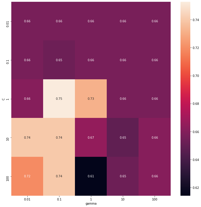
1 | sv_clf_rbf = SVC(kernel='rbf',random_state=1,C=1, gamma = 0.1) |
10-fold cross validation mean method scores for RBF SVM:0.763As can be seen from the grid search, the SVM with RBF kernel and hyperparameter C: 1, gamma 0.1 could achieve the highest performance
1 | linear_score = np.array(results_linear.mean_test_score) |
| 25 | 26 | 27 | 28 | 29 | |
|---|---|---|---|---|---|
| mean_fit_time | 0.0021414 | 0.00199142 | 0.00196731 | 0.00795052 | 0.0434071 |
| std_fit_time | 0.000204684 | 0.0003023 | 0.000284892 | 0.00302314 | 0.010914 |
| mean_score_time | 0.000635695 | 0.000739121 | 0.000567961 | 0.000703764 | 0.000822139 |
| std_score_time | 0.000104189 | 0.000289296 | 9.88127e-05 | 8.55103e-05 | 0.000257763 |
| param_C | 0.01 | 0.1 | 1 | 10 | 100 |
0.7358695652173913In the meantime, the best performance in linear model is 0.73587, and the mean_test_score in c =1,10,100 is relative similar. The influence of hyperparameter C are not significant. Apart from that the SVC function only provide
1 | ### Hyperparameter tuning for linear SVM (penalty, loss, C) |
1 | parameters = {'penalty':['l1', 'l2'], 'loss':['hinge', 'squared_hinge'],'C':[1, 10,100]} |
Best cross validation accuracy: 0.75
Test set score: 0.80
Best parameters: {'C': 10, 'loss': 'squared_hinge', 'penalty': 'l2'}
The test score of linear svm (test set score:0.80) still could not compete with the rbf kernel (test set score: 0.87), therefore, I would still insist on the SVM with RBF kernel and hyperparameter C: 1, gamma 0.1
1 | from sklearn.metrics import plot_confusion_matrix, confusion_matrix |
Training and validation loss
1 | print("Training loss is: {}".format(round(model.score(X_train,y_train),2))) |
Training loss is: 0.78
Testing loss is: 0.83
1 | train_mse = mean_squared_error(y_train,y_pred_train) |
The MSE value of training sample is: 0.22
The MSE value of testing sample is: 0.17
The training loss in SVM with RBF kernel in hyperparameter C: 1, gamma 0.1 is 0.78, with testing loss equals 0.83
The MSE value for training and testing in SVM with RBF kernel is 0.22 and 0.17 accordingly
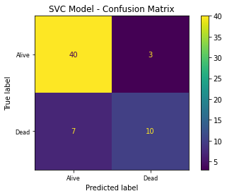
Plot the confusion matrix plot
1 | # confusion = confusion_matrix(y_test,y_pred) |
Evaluate the performance of the final selected model performance with respect to the chosen performance matrix
Accuracy:
$$\frac{TP+TN}{TP+TN+FP+FN}$$
Total:
$$Total = TP+TN+FP+FN$$
Precision:
$$\frac{TP}{TP+FP}$$
Recall:
$$\frac{TP}{TP+FN}$$
1 | from sklearn.metrics import classification_report |
                  precision    recall  f1-score   support

Heart Not Failed       0.85      0.93      0.89        43
      Heart Fail       0.77      0.59      0.67        17

        accuracy                           0.83        60
       macro avg       0.81      0.76      0.78        60
    weighted avg       0.83      0.83      0.83        60
ROC curve
AUC = Area under the curve
1 | from sklearn.metrics import confusion_matrix, plot_confusion_matrix, plot_roc_curve, plot_precision_recall_curve |
<sklearn.metrics._plot.roc_curve.RocCurveDisplay at 0x7fdff1de91f0>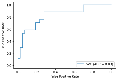
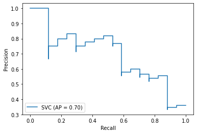
PR-curve
AP = Average Precision, summarizes such a plot as the weighted mean of precisions achieved at each threshold, with the increase in recall from the previous threshold used as the weight:
$$ AP =\sum_{N}(R_n-R_{n-1})P_n$$
where and are the precision and recall at the nth threshold. A pair is referred to as an operating point.
1 | plot_precision_recall_curve(model,X_test,y_test) |
Summary of the results
- Grid search to find the best hyperparameters in optimization of the model
- ten-fold cross validation used to evaluate machine learning models on a limited data sample
- SVM with RBF kernel and hyperparameter C: 1, gamma 0.1 would be the best performed model
- precision, recall, f1-score, accuracy value were applied and summarized in the previous table
- train loss and validation loss were 0.78 and 0.83 accordingly
- MSE value of training sample and testing sample is 0.22 and 0.17 accordingly
- No overfitting or underfitting problem observed because regularization method, cross-validation method were used to mitigate the potential problems
- The overall model is robust and in good generalization ability
- ROC curve and PR curve were visualized to demonstrate the final results; AUC is 0.83 and AP is 0.7
Conclusion and future work
In this project, I compared and devised a RBF SVM machine learning model for the prediction of heart failure. I firstly conducted a preliminary analysis of the whole dataset and utilized the PCA method to visualize the distribution condition of the samples. The initial analysis was not robust and precise, which required me to optimize the model. Then, I conducted feature selection to return the top 4 most correlated feature with the death event. Apart from that, I also compared the difference between normalization method as well as the validation methods. The final determined methods were to use four selected features (‘serum_creatinine’,’age’,’ejection_fraction’, ‘creatinine_phosphokinase’), StandardScalar methods and ten-fold cross validation to conduct the prediction. In addition, I also conduct the explorative data analysis to have a view of the selected feature. Furthermore, the PCA condition after feature selection still could not determine whether the dataset is linearly seperable or not, I, therefore, used the grid serach to return the most suitable hyperparameters. The final results suggested that the SVM with RBF kernel in gamma equals 0.1 and penalty C equals 1 could achieve the best performance. After that, the model performance was evaluated from confusion matrix, accuracy, precision, recall, f1-score. Moreover, the ROC plot and PR-curve plot with AUC and AP accordingly were indicated. The final accuracy could achieve 0.83, which is satisfactory.
In the future, since this project only used SVM related algorithms, I would like to incorporate more complicate algorithms, for instance, XGboost. Furthermore, the model’s interpretability are not great enough, and that would be my focus in the future.
Bibliography
Heart Fail:Analysis and Quick-prediction | Kaggle. (n.d.). Retrieved January 8, 2021, from https://www.kaggle.com/nayansakhiya/heart-fail-analysis-and-quick-prediction
Heart Failure - Model Prediction Comparisons (95%) | Kaggle. (n.d.). Retrieved January 8, 2021, from https://www.kaggle.com/rude009/heart-failure-model-prediction-comparisons-95
Heart Failure Prediction (AUC: 0.98) | Kaggle. (n.d.). Retrieved January 8, 2021, from https://www.kaggle.com/ksvmuralidhar/heart-failure-prediction-auc-0-98
Pedregosa et al., Scikit-learn: Machine Learning in Python, JMLR 12, pp. 2825-2830, 2011.
Other resources to download the code
Kaggle:
https://www.kaggle.com/yuxuanwu17/eda-of-heart-failure-and-optimization-of-svm
Github:
https://github.com/yuxuanwu17/kaggle/blob/main/Final_report.ipynb
- Post title:Heart failure detection by SVM-based machine learning model
- Post author:Yuxuan Wu
- Create time:2021-01-24 08:11:26
- Post link:yuxuanwu17.github.io2021/01/24/YuxuanWu-1716309-INT305-Report/
- Copyright Notice:All articles in this blog are licensed under BY-NC-SA unless stating additionally.